
One of the benefits of Bayesian model-informed precision dosing (MIPD) is that it can reduce the number of drug levels you need. That’s good for patients — fewer blood draws — and good for clinical workflows and operation budgets.
Overall, research from our Data Science team and from other research groups suggests that:
- Bayesian MIPD can accurately dose busulfan with fewer samples than traditional approaches
- Sample timing still matters, even when the sample count is reduced
Still, if you’re used to tools that require a full set of precisely timed levels, switching to sparse sampling can feel risky. A question we hear all the time for sites considering MAP Bayesian for busulfan dose personalization is:
“Can I really use just four samples?”
In this post, we’ll look at recent evidence in busulfan dosing to help answer that question, and why fewer samples don’t necessarily mean less confidence.
Why busulfan requires personalized dosing
Busulfan is a key component of conditioning regimens for gene therapies and hematopoietic stem cell transplantation. However, busulfan dosing is challenging due to its narrow therapeutic index. Too little exposure increases the risk of graft failure and relapse. Too much increases the risk of severe toxicity and transplant-related mortality.
For busulfan, the best predictor of both efficacy and toxicity is the cumulative exposure, measured as the area under the concentration-time curve (AUC). For best outcomes, aim for a cumulative AUC between 78–101 mg×h/L.
Patients vary considerably in how they process busulfan, even when given the same dose. As a result, reliably hitting this target requires individualized dosing rather than relying on fixed dosing. For more information, see our previous post about using MIPD for bone marrow conditioning regimens.
The traditional approach: effective, but sampling-heavy
Historically, busulfan AUC has been estimated using non-compartmental analysis (NCA), which estimates exposure by plotting measured drug levels over time, connecting them with trapezoids, and summing the area under the resulting curve.
NCA is appealing because it’s relatively straightforward and data-driven, as it doesn’t rely on a pharmacokinetic model. But there’s a tradeoff: it’s very sampling intensive.
In routine clinical practice, NCA-based workflows often require 6–7 samples per dosing interval and strictly-timed draws.
This works — but it’s burdensome for patients and staff.
Bayesian MIPD: efficacy without the sampling burden
Bayesian MIPD takes a different approach. Instead of treating each patient as a blank slate, it starts with what we already know: a population PK model that describes how busulfan behaves across patients.
Patient-specific busulfan levels are then used to individualize that model — updating model parameters like clearance and volume estimates for the individual patient.
Because prior knowledge and patient data are combined, Bayesian approaches can estimate exposure accurately with fewer samples than NCA, which is entirely data-driven.
How do NCA and Bayesian approaches compare for busulfan MIPD?
To answer this, we first turned to simulation. Simulations let us test different sampling strategies across thousands of “digital patients” without running costly prospective trials. Just as importantly, they let us separate two things that are easy to conflate in clinical practice: the exposure a patient actually experiences, and the exposure we estimate based on measured levels.
In a simulation, we know the true exposure because the drug concentrations are generated from a known model. That means we can calculate each patient’s actual AUC exactly, and then test how well different methods estimate that exposure when they only see a limited number of noisy, clinically realistic samples.
We compared two approaches:
- Dose adjustment based on NCA
- Dose adjustment based on MAP Bayesian estimates
At first glance, both methods appeared to work very well. Nearly all patients were estimated to be within the AUC target range according to the AUC estimation method used.
But when we looked at true exposure — the actual AUC experienced by our simulated patients, rather than what the estimation methods reported — we found something surprising:
Patients dosed using NCA appeared to hit the target 98.7% of the time — yet their true cumulative AUC was within range only 65% of the time. In other words, NCA often gave a false sense of confidence.
The story was different for Bayesian MIPD. Estimated target attainment was similarly high (99.9%), but true target attainment was much closer to that estimate (92.1%), in part because Bayesian models account for drug elimination during the infusion period, whereas trapezoidal NCA implicitly assumes the body is not eliminating drug during infusion.
(For more on why this happens, see our blogpost on NCA versus MAP Bayesian methods.)
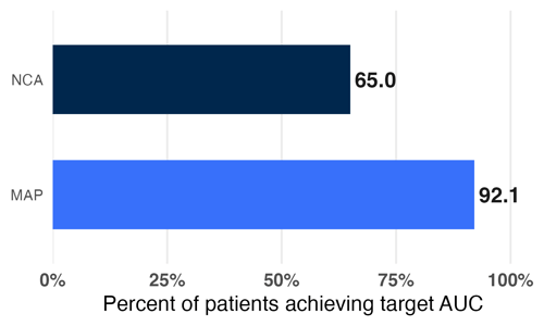
Figure 1: Proportion of simulated patients achieving a true cumulative AUC within 15% of the target, using MAP Bayesian estimation or NCA for dose individualization. Adapted from Hughes et al., J PKPD (2024).
How few samples is “too few”?
We also looked at how Bayesian performance changed as sample count decreased.
- Five samples led to ~93% true target attainment
- Reducing to three samples still achieved ~91–92% target attainment
- Bayesian methods and limited sampling strategies (91-93%) led to higher target attainment than NCA and dense sampling (68%)
In other words, performance was surprisingly robust to fewer samples.
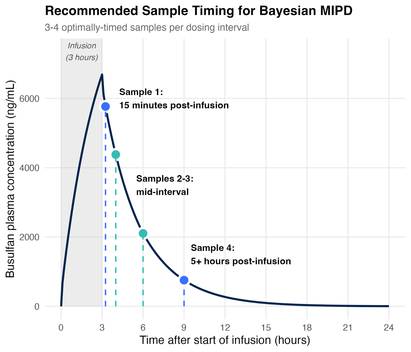
That said, timing still matters. The most informative strategies included:
- One sample shortly after the end of infusion: this gives us insight into volume of distribution
- One late sample (around 5 hours after the end of infusion): this is important for accurately estimating clearance
- One or two mid-interval samples: these help us further refine our estimates of individual PK parameters
A more detailed explanation of these results was also recently published by our team in J PKPD.

Figure 2: Four well-timed samples suffice for MAP Bayesian estimation. Schematic showing recommended sampling times based on simulations and a review of real-world evidence.
While samples collected at these time points are the most informative, Bayesian methods can still make effective use of samples collected at any time point, whereas NCA is more sensitive to mis-timed samples.
What does real-world evidence show?
Simulation results are helpful, but what ultimately matters is how these approaches perform in real patients. Fortunately, multiple clinical studies have evaluated Bayesian AUC estimation and dosing using limited sampling — and the results are consistent.
Across different institutions, models, and patient populations, several studies have demonstrated that three to four well-timed samples can be sufficient to estimate busulfan exposure accurately when using Bayesian methods.
For example, Neely et al. showed that MAP Bayesian estimation using just two optimally timed samples — 15 minutes and 4 hours after the end of infusion — produced AUC estimates within 5–12% of those obtained using NCA with nine samples. Importantly, there was no statistically significant bias. This study used a population model developed in the same patient cohort, which likely contributed to the strong performance. In more general clinical settings, using three to four samples remains a more conservative and widely applicable approach.
Other groups have reached similar conclusions. In a cohort of patients with dense sampling, Bullock et al. evaluated different limited sampling strategies and found that Bayesian estimates remained unbiased even when sample counts were reduced. A four-sample scheme was sufficient to characterize busulfan pharmacokinetics and support dose adjustment, suggesting that routine therapeutic drug monitoring does not require exhaustive sampling.
Beyond pharmacokinetic accuracy, some studies have also linked Bayesian-guided dosing with better clinical outcomes. Bleyzac et al. reported that dose adjustment based on three samples per interval (at 1, 2.5, and 5 hours after the end of infusion) led to higher rates of full engraftment at three months and a markedly lower incidence of veno-occlusive disease compared to a case-matched arm without dose adjustment.
More recent studies continue to support these conclusions. Protzenko et al. reported positive outcomes using Bayesian-guided dosing with three samples (15 minutes, 6 hours, and 9 hours after infusion), while Shukla et al. showed superior target attainment when dosing was guided by Bayesian estimates using four samples, compared to NCA-based adjustment.
Taken together, these studies reinforce a consistent message: Bayesian MIPD enables accurate and effective busulfan dosing with limited sampling schemes, provided that samples are appropriately timed and a suitable population model is used.
What is right for my patients?
Across simulations and real-world studies, the evidence points in the same direction: Bayesian MIPD enables accurate busulfan dosing with fewer samples, without sacrificing confidence or patient safety. While careful sample timing remains important, limited sampling strategies can substantially reduce burden for patients and care teams while maintaining, or even improving, target attainment.
For transplant programs considering a move away from sampling-heavy workflows, these results help answer a common concern: fewer well-timed samples do not have to mean less confidence in patient care.
Interested in implementing MIPD for transplant and cellular therapy? Learn more about our BMT conditioning agent modules below.
